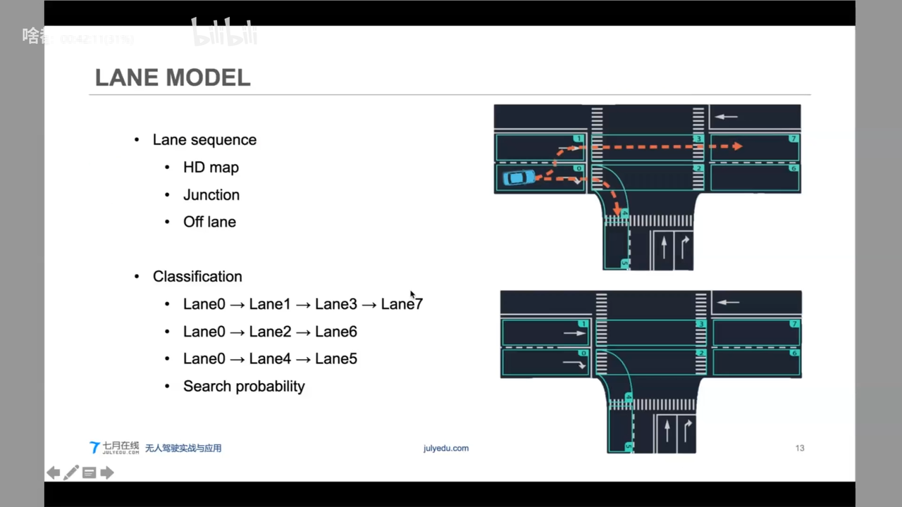
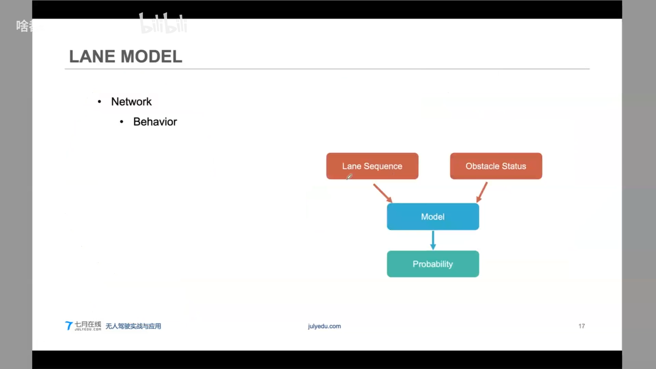
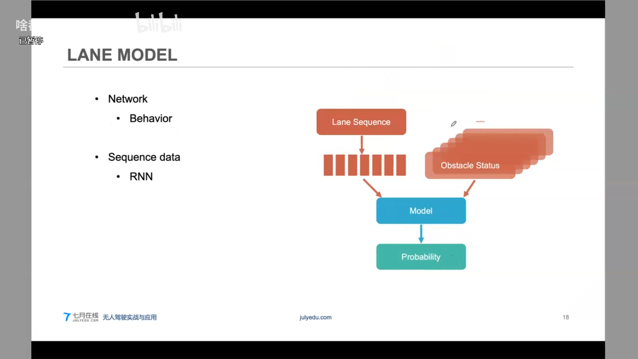
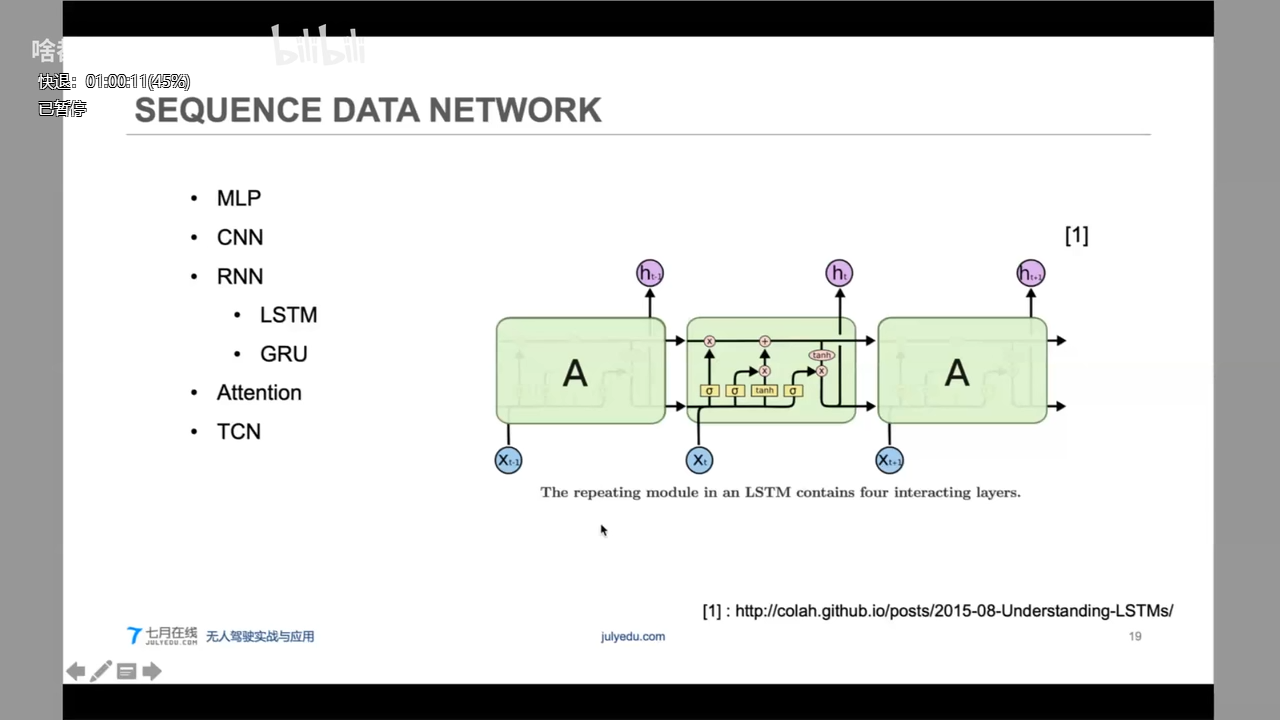
Contents:
[TOC]
Naikai RL
1、基本原理,概念
依赖模型:
策略更新方法:
- 基于值函数的强化学习,
- 基于直接策略搜索的强化学习,
- Actor-Critic的方法。
根据回报函数是否已知分为:正向强化学习和逆向强化学习
正向强化学习:从回报(reward)学到最优策略
逆向强化学习:从专家示例中学到回报函数
根据任务大小和多少分为:分层强化学习、元强化学习、多智能体强化学习、迁移学习等
发展趋势
\1. 贝叶斯强化学习
融合推理能力,可解决POMDP问题
\2. 分层强化学习
解决大规模学习问题
\3. 元强化学习
解决对任务学习
\4. 多智能体强化学习
博弈:合作,竞争,混合
路线图
强化学习课程的路线图
\1. 搞清楚马尔科夫决策过程的概念
\2. 抓住强化学习的基本迭代过程:策略评估和策略改善
\3. 掌握强化学习最常用的两种方法:基于值函数的方法和基于直接策略搜索的方法
\4. 强化学习的其他方法:AC框架,基于模型的强化学习,基于记忆的强化学习等等
置信度算法
多臂赌博机:UCB https://blog.csdn.net/chenxy_bwave/article/details/121715210
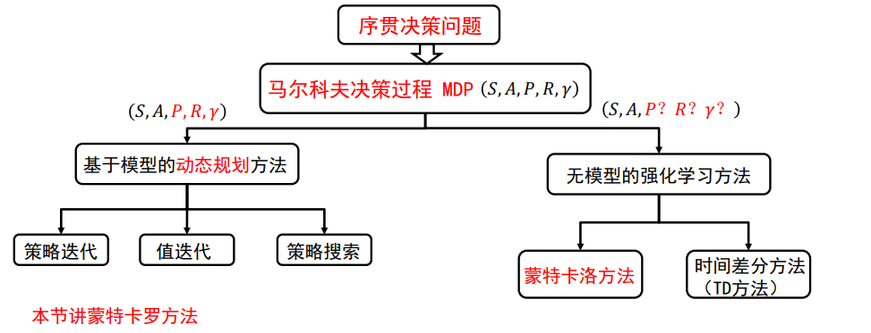
2、马尔可夫决策过程
有限马尔可夫决策问题的三种基本方法:
马尔科夫性
马尔科夫性: 系统的下一个状态只与当前状态有关,与以前状态无关。
定义:一个状态St是马尔科夫的,当且仅当:
$$
𝑃 [𝑆_{𝑡+1 }| 𝑆_𝑡] = 𝑃 [𝑆{𝑡+1}|𝑆_1, ⋯ , 𝑆_𝑡]
$$
- 当前状态蕴含所有相关的历史信息
- 一旦当前状态已知,历史信息将会被抛弃
马尔可夫决策过程(MDP)
MDP:带有决策和回报的马尔科夫过程:
定义:马尔科夫决策过程由元组: $(𝑆, 𝐴, 𝑃, 𝑅, \gamma)$ 描述S为有限的状态集,A为有限的行为集,P为状态转
移概率,R为回报函数,𝛾为折扣因子 ;
随机变量 s’,r的分布由条件概率定义:
$$
p(s’, r| s,a) = Pr{ S_t=s’, R=r|S_{t-1}=s, A_{t-1} = a }
$$
值函数与策略
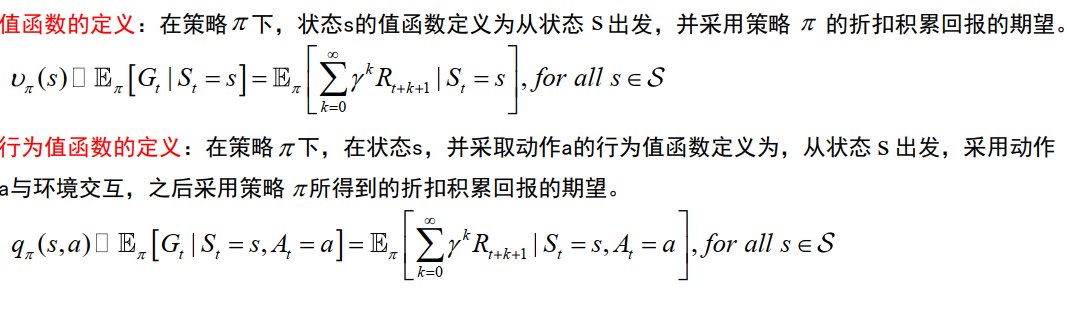
状态s的好坏:值函数 V(s ) (状态的函数)。
值函数跟策略有关,不同的策略对应不同的值函数
策略的定义:
一个策略 𝜋是给定状态s时,动作集上的一个分布:
$$
\pi(𝑎|𝑠) = 𝑝[𝐴_𝑡 = 𝑎 | 𝑆_𝑡 = 𝑠]
$$
策略的定义
值函数的定义
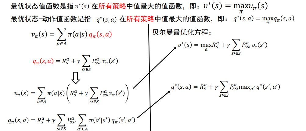
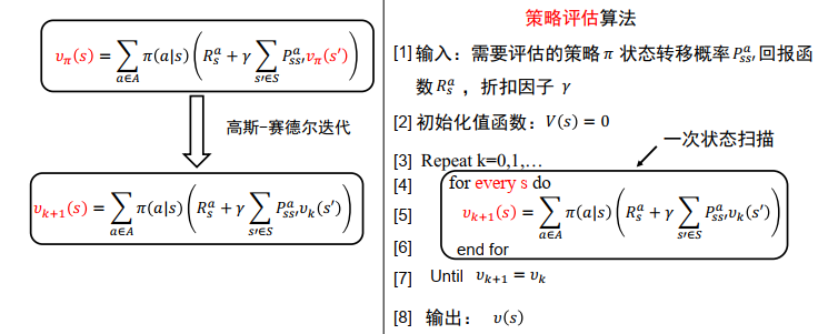
马尔科夫决策过程:贝尔曼方程
$$
v_{\pi}(s) = \sum_{a\in A} \pi(a|s)(R_s^a + r\sum_{s’\in S} P_{ss’}^a v_{\pi}(s’) )
$$

最优价值函数和最优状态-动作值函数
3、动态规划到强化学习
单阶段决策:数学规划
多阶段决策:动态规划
动态规划的本质:将多阶段决策问题通过贝尔曼方程转化为多个单阶段的决策问题
离散贝尔曼方程:
连续贝尔曼方程:
微分动态规划方法
DP -> RL
控制领域集中于连续高维问题
最优控制:模型已知,立即回报解析地给出,状态空间小。
近似动态规划:利用机器学习方法学习值函数,解决维数灾难
计算机领域:集中于离散大规模问题
以马尔科夫决策过程为基础,强化学习 无模型,回报函数不解,状态空间无穷
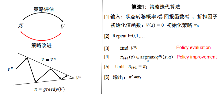
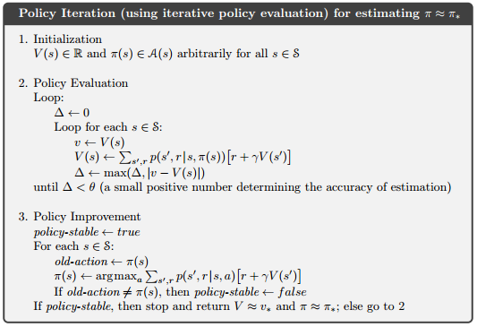
动态规划: 策略评估(估计值函数) ,策略改进
所有强化学习算法都可以看成是动态规划算法,只是用更少的计算,并且没有假设完美模型
策略评估(Prediction)
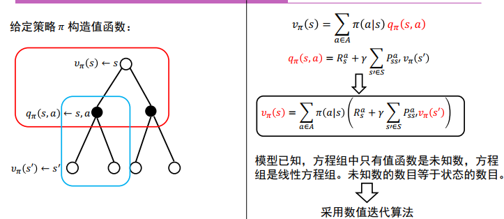
策略改进

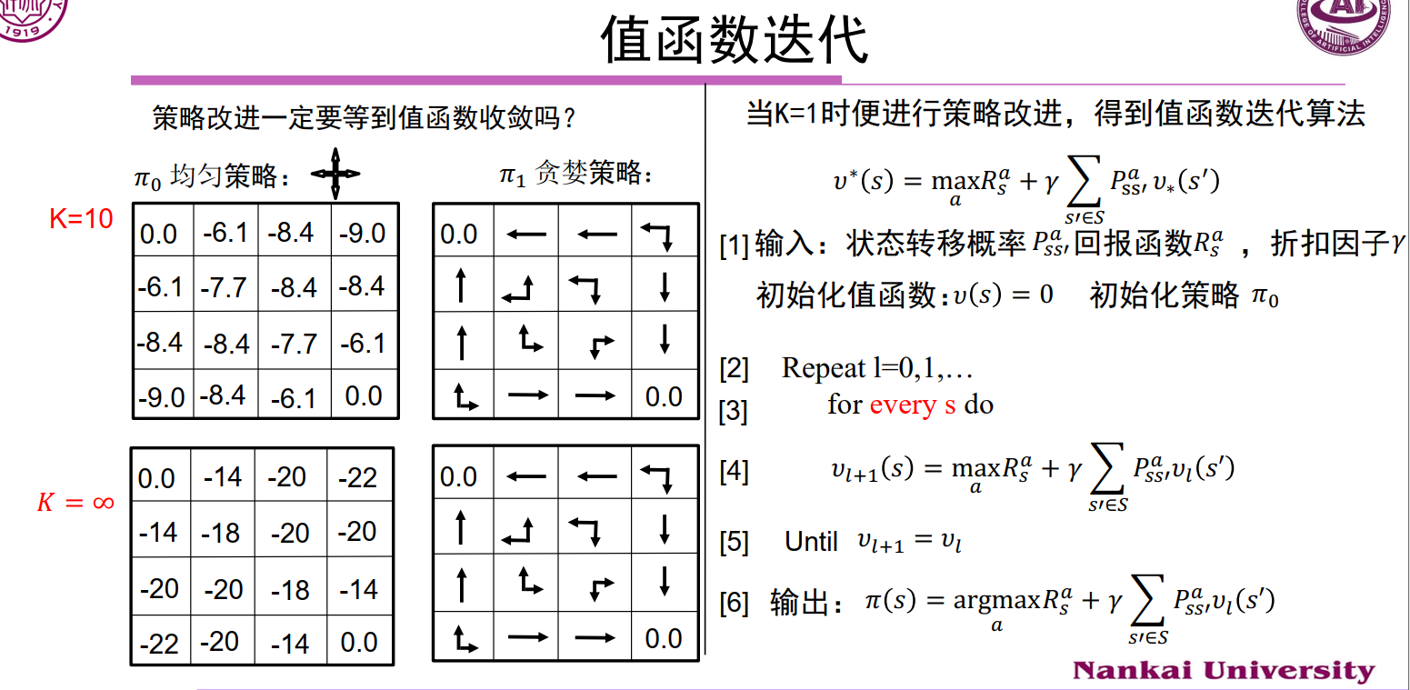
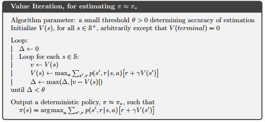
值函数迭代
4、MC & TD
值函数:
$$
v_{\pi}(s) = E_{\pi} [G_t|S_t=s]= E_{\pi}[\sum_{k=0}^{\infty} r^kR_{t+k+1} | S_t=s]
$$
状态-行为值函数:
$$
q_{\pi} = \sum_{a\in A} \pi(a|s)\Big(R_s^a + r\sum_{s’ \in S} P_{ss’}^a v_{\pi}(s’)\Big)
$$
RL_Sutton
2、Multi-armed Bandits
3、Finite Markov Decision Processes
4、DP
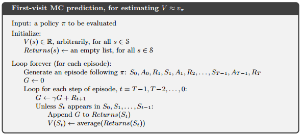
5、MC
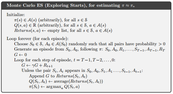
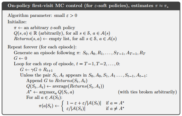
5.3 MC (ES)
5.4 On-Policy
On-policy methods attempt to evaluate or improve the policy that is used to make decisions;
off-policy methods evaluate or improve a policy different from that used to generate the data.
基于experience replay的方法基本上都是off-policy的。
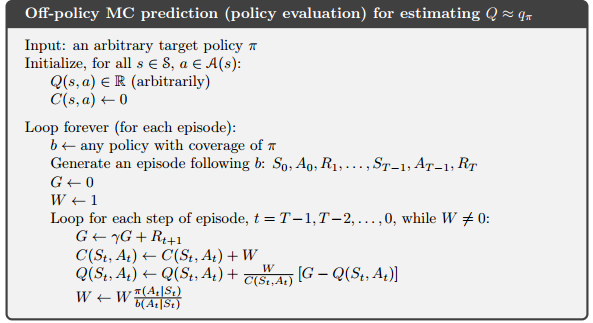
5.5 Off-policy
target policy : to learned
behavior policy : to generate behavior
- 行为策略(behavior policy):agent与environment交互使用的策略,用来产生数据来改进agent的行为。因为需要有探索性,这个策略是随机的。
- 目标策略(target policy): 学成以后用于应用的策略。这个时候agent根据这个策略来采取行动。
on-policy 是Off-policy的一种特例(same)
5.6 Incremental Implementation
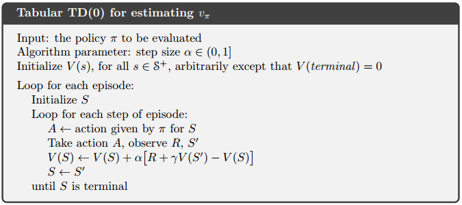
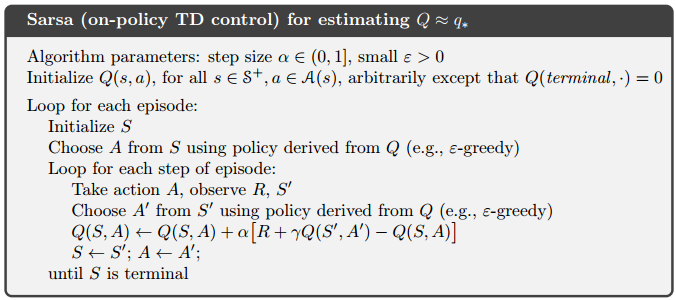
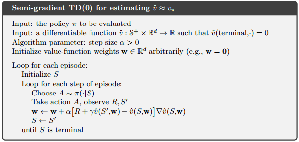
6、TD
TD(0)
Sarsa(on-policy TD)
TD(0)学习的是状态价值函数V(s),这里因为(),所以需要学习动作价值函数Q(s,a);
五元组$(S_t, A_t, R_{t+1}, S_{t+1}, A_{t+1})$
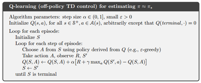
Q-learning (off-policy TD)
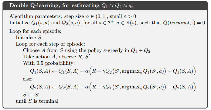
Double Q-learning
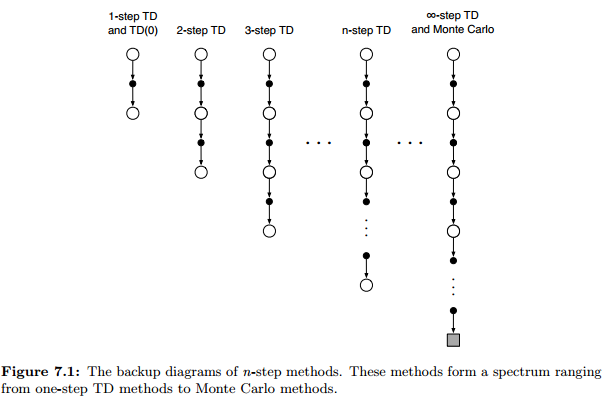
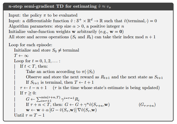
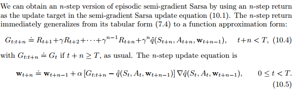
7、n-step Bootstrapping
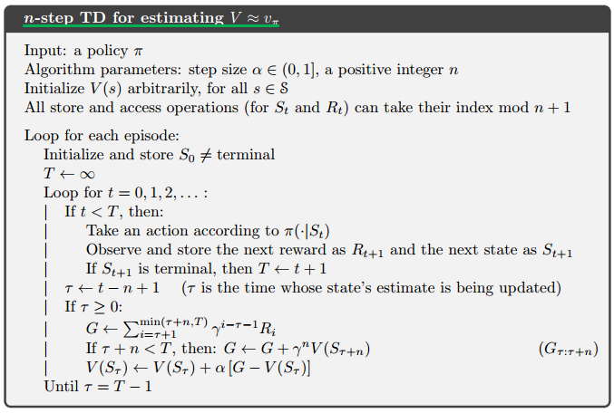
7.1 n-step TD
各个算法的更新目标(回报)
$$
\begin{align*}
& MC: G_t = R_{t+1} + \gamma R_{t+2} + \gamma^2 R_{t+3} + … + \gamma^{T-t-1} R_T \
& TD(0): G_{t:t+1} = R_{t+1} + \gamma V(S_{t+1}) \
& \gamma V(S_{t+1})= \gamma R_{t+2} + \gamma^2 R_{t+3} + … + \gamma^{T-t-1} R_T\
& TD(2): G_{t:t+1} = R_{t+1} + \gamma R_{t+2}+ \gamma^2 V(S_{t+2}) \
& TD(n): G_{t:t+n} = R_{t+1} + \gamma R_{t+2}+ …
+ \gamma^{n-1} R_{t+n} + \gamma^{n} V_{t+n-1}(S_{t+n}) \tag{7.1}
\end{align*}
$$
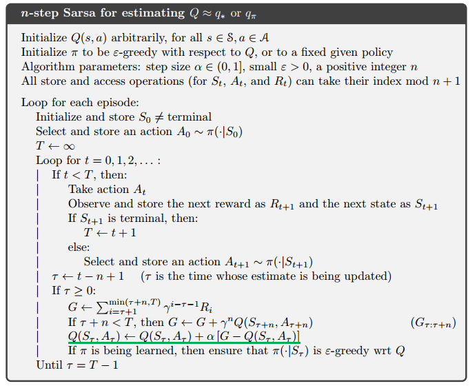
n-step Sarsa
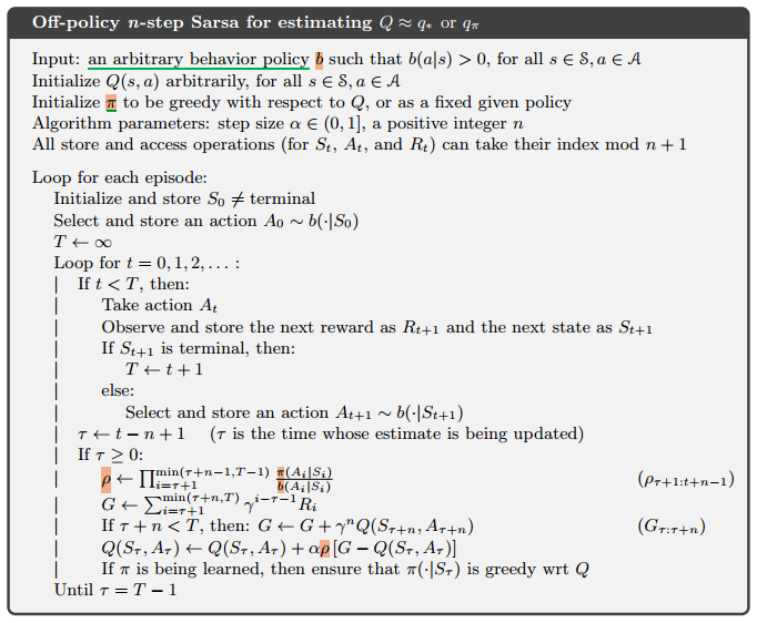
n-step Sarsa(Off-policy)
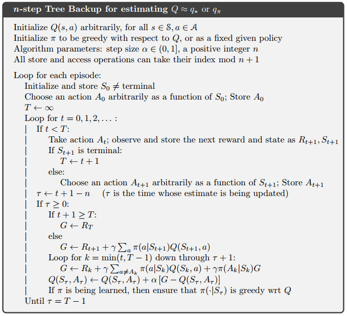
n-step Tree Backup
8、 Planning and Learning with Tabular Methods
9 On-Policy Prediction
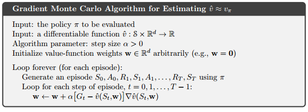
9.1 Value-function Approximation
$$
\begin{align*}
& MC: S_t \rightarrow G_t \
& TD(0): S_t \rightarrow R_{t+1} + \gamma\hat{v}(S_{t+1}, W_t) \
& TD: S_t \rightarrow G_{t:t+n} \
& DP: S_t \rightarrow E_\pi[R_{t+1} + \gamma\hat{v}(S_{t+1}, W_t) | S_t = s]
\end{align*}
% & 左对齐
$$
9.2 The Prediction Objective
预测目标: Mean Squared Value Error 均方差

9.3 Stochastic-gradient and Semi-gradient TD(0) Methods
随机梯度与半梯度方法
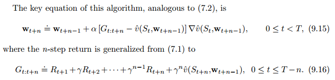
9.4 Linear Methods(n-step Semi-Graditent TD)
n-step Semi-Graditent TD
9.5 Feature Construction for Linear Methods
Polynomials 多项式
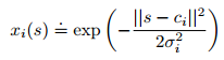
Radial Basis Functions 径向基函数
与其说 ,特征0,1;不如说是区间[0,1]之间的任何东西,反应特征存在的不同程度;
RBF特征采用高斯表示,当前状态s和中心(原型)状态ci之间的举例表示;
9.7 ANN (非线性函数逼近)
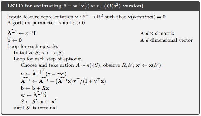
9.8 LSTD
Least-Squares TD
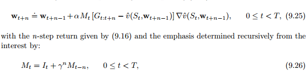
9.11 Looking Deeper at On-Policy Learning : Interest and Emphasis
(9.15)引入强调值Mt
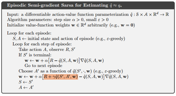
10 On-Policy Control
10.1 Episodic Semi-gradient Control
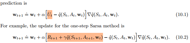
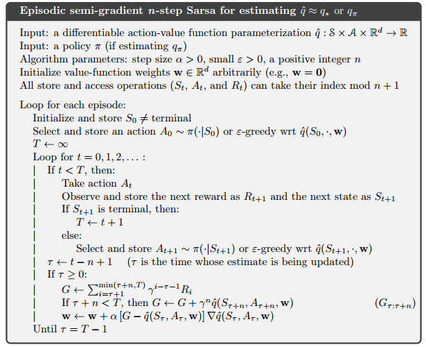
10.2 Semi-gradient n-step Sarsa
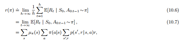
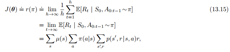
10.3 Average Reward: A New Problem Setting for Continuing Tasks

10.4 Deprecating the Discounted Setting
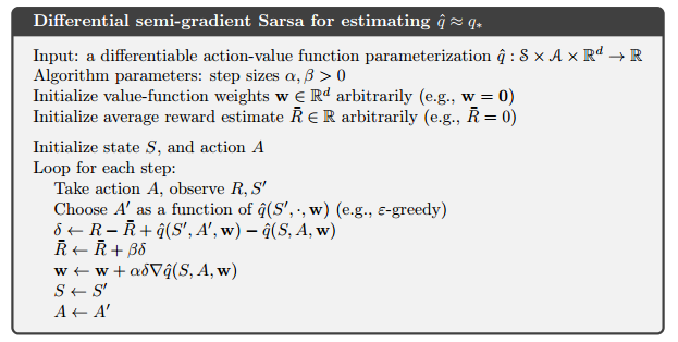
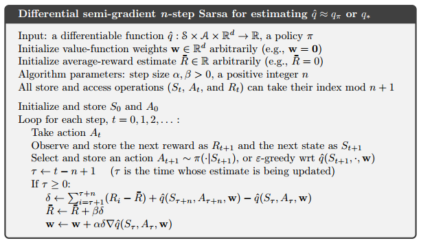
10.5 Differential Semi-gradient n-step Sarsa
11 Off-Policy Methods
12 Eligibility Traces 资格迹
12.1 $\gamma 回报$
参数化的函数逼近:
$$
G_{t:t+n} = R_{t+1} + \gamma R_{t+2}+ …
+ \gamma^{n-1} R_{t+n} + \gamma^{n} V_{t+n-1}(S_{t+n}, W_{t+n-1}) \tag{12.1}
$$
$\lambda$ 回报:
$$
G_t^{\lambda} = (1- \lambda) \sum_{n=1}^{\infty} \lambda^{n-1}G_{t:t+n} \tag{12.2}
$$
提取终止项:
$$
G_t^{\lambda} = (1- \lambda) \sum_{n=1}^{T-t-1} \lambda^{n-1}G_{t:t+n}
+ \lambda^{T-t-1}G_{t} \tag{12.3}
$$
更新目标:
$$
w_{t+1} = w_{t} + \alpha[ G_{t}^{\lambda} - \hat{v}(S_t, w_t)]
\nabla \hat{v}(S_t, w_t), t=0,…,T-1 \tag{12.4}
$$
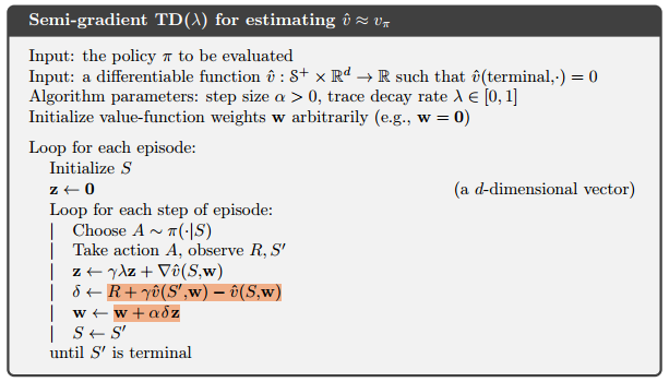
12.2 TD($\lambda$)
每一步都更新权重向量(原本是结束时更新)
计算平均分布在整个时间轴,而不是结束时
也适用于持续性问题,(episode更不用说了)
资格迹$z_t$,短期记忆;是一个和权值向量w_t同维度的向量;
- 唯一作用:影响权值向量,进而权值向量影响估计值v;
权值向量$w_t$:长期的记忆
$$
\begin{align*}
& z_{-1} = 0,\
& z_t = \gamma \lambda z_{t-1} + \nabla \hat{v}(S_t, w_t), 0 \leqslant t \leqslant T
\tag{12.5}
\end{align*}
$$
$$
\begin{align*}
& \delta_t = R_{t+1} + \gamma \hat{v}(S_{t+1}, w_t) - \hat{v}(S_t, w_t) \tag{12.6} \
& w_{t+1} = w + \alpha \delta_t z_t \tag{12.7}
\end{align*}
$$
12.3 n-step Truncated $\lambda$-return Methods
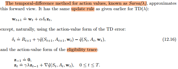
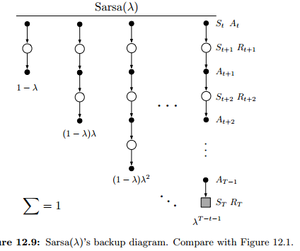
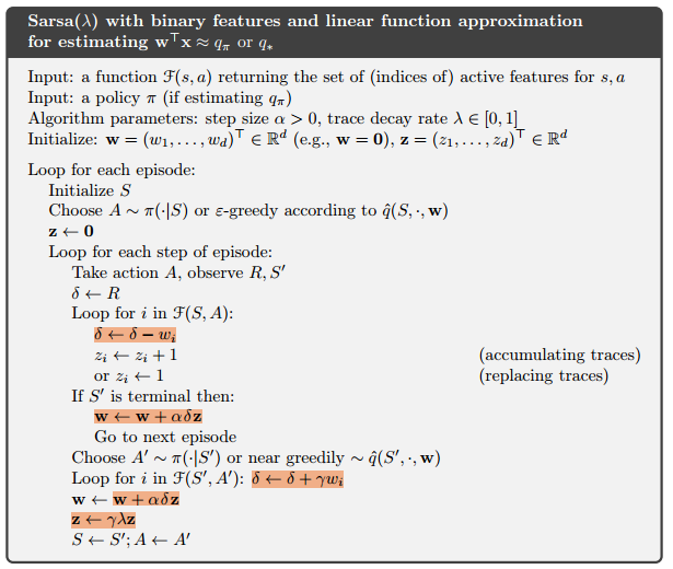
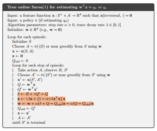
12.7 Sarsa()
Sarsa: TD metod for action values;
extend eligibility-traces to action-value methods.
learn approximate action values, qˆ(s, a, w), rather than approximate state values, vˆ(s,w)


12.8 Variable $\lambda$ and $\gamma$
13 Policy Gradient Methods
参数化的策略方法;价值函数仍可用于学习策略的参数,但是对于动作选择而言,就不是必须了。
梯度上升:gradient ascent in J。
$$
\theta_{t+1} = \theta_t + \alpha \widehat{ \nabla J(\theta_t) } \tag{13.1}
$$
同时学习策略和值函数的近似值的方法通常称为 演员-评论家方法,其中“演员”是指所学策略,而“评论家”是指所学习的值函数,通常是状态价值函数。
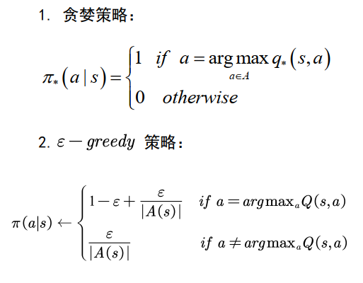
1. Policy Approximation and its Advantages
动作偏好soft-max (soft-max in action preferences)
例如在扑克中诈(bluffing)。 动作值方法没有找到随机最优策略的自然方法,而策略逼近方法却可以,如示例13.1所示。
相比于动作值参数化,策略参数化可能具有的最简单的优势是策略可能是一种做近似更简单的函数。 问题的策略和行动价值函数的复杂性各不相同。
优势1:近似策略接近于一个确定策略;
优势2:可以以任意概率选择动作;
- 例如,在信息不完美的纸牌游戏中,最佳玩法通常是用特定的概率做两件不同的事情,比如在扑克中虚张声势。
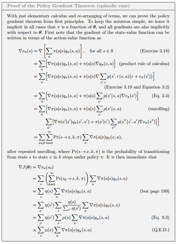
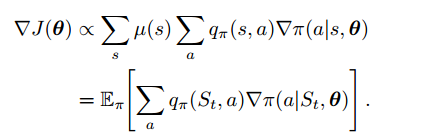
2. The Policy Gradient Theorem(定理)
策略参数化选择动作的概率会平滑的变化,这很大程度上导致了其更强的收敛保证。
特定(非随机)状态下开始:
$$
J(\theta) = v_{\pi_\theta}(s_0)
$$
3. REINFORCE: Monte Carlo Policy Gradient
回想我们前几节提到的梯度上升,我们只需要一种获取样本的获取方法,让采样样本的梯度近似或者等于策略梯度:
- 样本梯度的期望 正比于 实际梯度(作为参数的函数的性能度量)
策略梯度定理公式:
这时我们可以应用梯度上升算法(13.1):

由于更新涉及了所有的动作,因此被称为全部动作算法,不过,我们更关注在时刻t被采样的动作,因此需要用策略对动作进行期望加权:
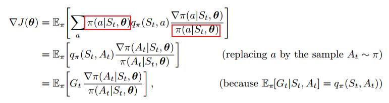
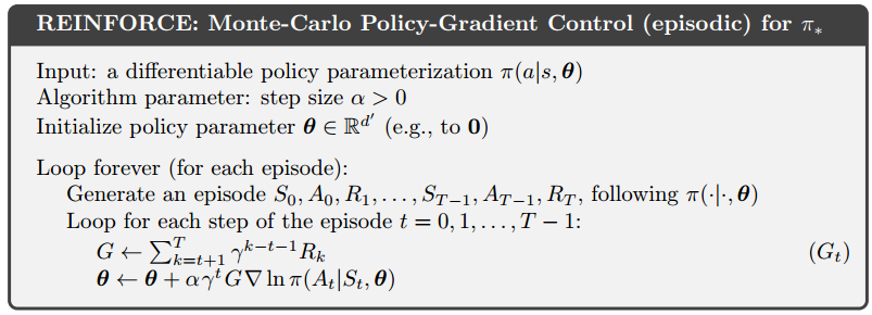
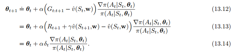
使用这个算法进行梯度上升,就可以得到我们想要的Reinforce算法:
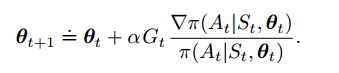 (13.8)
综合起来,就可以写出算法伪代码:
$$
\nabla ln(x) = \frac{\nabla x}{x}
$$
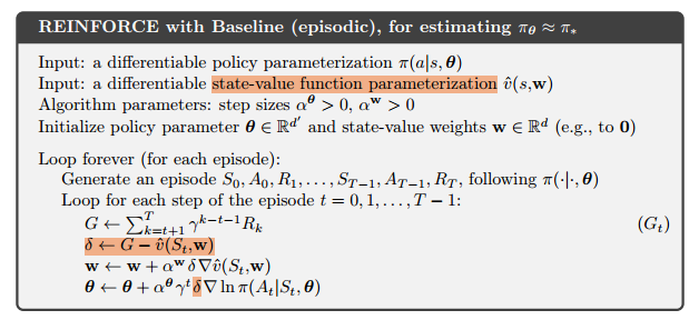
4、带有baseline的Reinforce
可以在动作价值函数后加一个对比的baseline(v(s))以推广策略梯度定理,只要不随动作a变化就行:

为什么可以这么做呢?因为对策略求和的梯度为0:
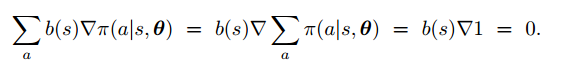

比较自然的一个baseline就是状态价值函数了。这样做的好处在于,在不改变期望的前提下,大大降低了方差。
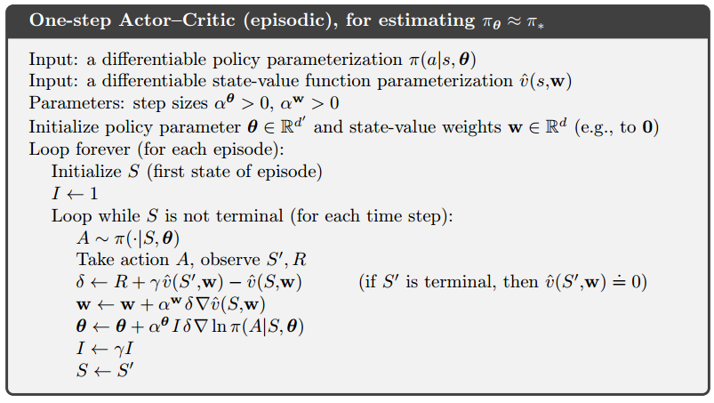
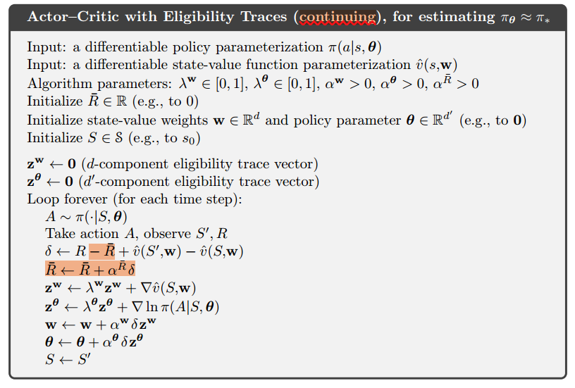
5. Actor–Critic Methods
尽管带baseline的强化学习方法学习了一个状态价值函数,我们也不能说它是演员评论家(actor critic)方法,因为状态价值函数仅仅当做baseline,而不是Critic。没有被用作自举(bootstrapping,根据后续状态的估计值更新状态的值估计)。
然而,和所有MC方法一样,这种方法收敛很慢,而且难以在线实现。
use actor–critic methods with a bootstrapping critic.
为了解决这个问题,我们引入TD(0)方法与演员评论家方法:
这是一个online、增量式的算法,所有收集到的数据只会在第一次使用,之后就弃用:
n-step (+资格迹)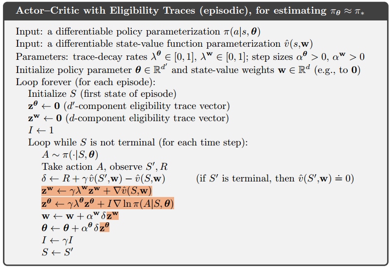
6、持续性问题的策略梯度
Policy Gradient for Continuing Problems

7、Policy Parameterization for Continuous Actions
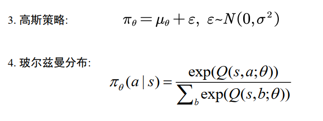
通过学习概率分布的统计量,而不是每一个动作的概率,我们能够解决连续动作空间的任务正态分布的概率密度函数: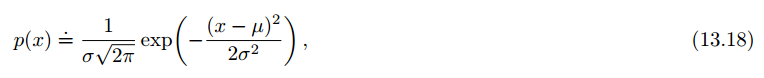
为了得到参数化的策略函数,我们不如把策略定义为正态分布的概率密度:

我们分别用均值和标准差来近似策略参数向量,由于标准差为正数,所以得用指数形式:

参考资料
《南开大学–强化学习课程PPT》
《强化学习 Sutton》
★★★★十二、Policy Gradient Methods 策略梯度方法
强化学习 (Reinforcement Learning) | 莫烦Python