[TOC]
Algorithm Impl CV/CG Transform
Transform
[TOC]
angle2matrix
1 | def angle2matrix(angles): |
angle2matrix_3ddfa
1 | def angle2matrix_3ddfa(angles): |
—————————————— 1. transform(transform, project, camera).
———- 3d-3d transform. Transform obj in world space
rotate
1 | def rotate(vertices, angles): |
normalize
1 | ## -------------- Camera. from world space to camera space |
lookat camera
1 | def lookat_camera(vertices, eye, at = None, up = None): |
orthographic_project 正交投影
1 | ## --------- 3d-2d project. from camera space to image plane |
perspective_project 透视投影
1 | def perspective_project(vertices, fovy, aspect_ratio = 1., near = 0.1, far = 1000.): |
to_image
1 | def to_image(vertices, h, w, is_perspective = False): |
estimate_affine_matrix_3d23d
1 | #### -------------------------------------------2. estimate transform matrix from correspondences. |
estimate_affine_matrix_3d22d
1 | def estimate_affine_matrix_3d22d(X, x): |
P2sRt
1 | def P2sRt(P): |
isRotationMatrix
1 | #Ref: https://www.learnopencv.com/rotation-matrix-to-euler-angles/ |
matrox2angle
1 | def matrix2angle(R): |
Algorithm Survey
[TOC]
算法类型
图形学算法
S,R,T
- Scala
- 旋转
- 位移
- 对齐 (mtcnn align 算法)
- 仿射变换 (CV-transformations.md)
- 线性插值
CG Algorithm (Algorithm-CG.md)
/home/simon/data/blogs/source/_posts/CV-3D-Transform.md
- LBS算法 (CV-3D-BuildModel-CMPL.md)
点云对齐算法
CV-3D-Base.md
统计机器学习算法
- k-means
数据降维
- PCA
数据降维基础
- 奇异值分解SVD
- 特征值分解EVD
游戏树算法
- minimax
- pn-search
- alpha-beta剪枝
增强学习算法
- MCTS
- UCT
- CFR
Algorithm CG
Python Lib OpenCV
[TOC]
OpenCV -API (python)
APi Tutorials
imgproc 模块. 图像处理 OpenCV 2.3.2 documentation
图像平滑(模糊)处理 blur /GaussianBlur / MedianBlur / BilaterFilter
腐蚀-膨胀
形态变换
一、Image I/O
imread
imsave
imshow()
resize
cv2.resize的第二个参数dim是(W, H)
1 | cv2.resize(array, (W, H)) |
copyMakeBorder
cv2.copyMakeBorder的第二个到第五个参数是top, bottom, left, right,是先H后W
opencv中以左上角为原点,W方向为x,H方向为y
1 | def copyMakeBorder(src, top, bottom, left, right, borderType, dst=None, value=None): # real signature unknown; restored from __doc__ |
**扩充src的边缘,将图像变大,**然后以各种外插方式自动填充图像边界,这个函数实际上调用了函数cv::borderInterpolate,这个函数最重要的功能就是为了处理边界,比如均值滤波或者中值滤波中,使用copyMakeBorder将原图稍微放大,然后我们就可以处理边界的情况了
CV demo {实现crop,pad)
使用opencv-python 对图像进行resize和填充
在图像输入神经网络之前,需要进行一定的处理,假设神经网络的图像输入是256 256然后进行了224 224的random crop。
我们需要进行如下处理:
读入原始图像
1 | image = cv2.imread("img.jpg") |
截取图像中有价值的部分
1 | region = image[y1:y2, x1:x2] |
确定图片的长边和短边,然后把长边resize到224,保持纵横比的情况下resize短边
1 | w, h = x2 - x1, y2 - y1 # h, w = image.shape |
把图片进行填充,填充到256 256
1 | W, H = 256, 256 |
图片在输入网络之后,训练的时候进行random crop,就会发生有一部分被截取掉的情况,而这正是我们想要的图像增强
在test阶段,是进行centre crop,而正好把整个图像都截取出来,而这正是我们想要的
值得注意的是,image.shape,cv2.resize和cv2.copyMakeBorder几个函数
image.shape的输出是(H, W, C)
三、形态变化
- 形态变化是基于图像中物体的形态进行一些简单变换,通常在二值化的图像上进行,
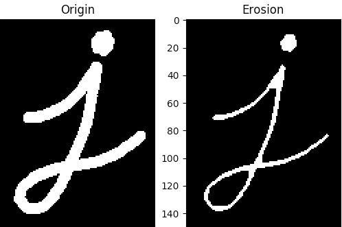
1.侵蚀
侵蚀的基本思想就像土壤侵蚀一样,侵蚀着物体前景色(白色)的边界。形态学处理内核在图像窗口中滑动,只有当内核下的所有像素都为1时,原始图像中的像素(1或0)才会被视为1,否则它将被侵蚀(变为零)。我要说话
因此最终的表现就是,所有靠近前景色边界的像素都将而被丢弃,内核尺寸越大丢的越多,即白色的区域会减小。这种操作对于消除小的白色噪声(如我们在色彩空间一章中所看到的)、分离两个连接的对象等非常有用。
1 | def pltShow(img): |
2.膨胀
膨胀的效果正好与侵蚀相反,如果内核下至少有一个像素为“1”,则像素元素为“1”。因此,它增加了图像中的白色区域(前景对象)的大小。我要说话
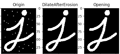
在去除噪音的时候,一般采用的操作是侵蚀之后再膨胀。侵蚀消除了白色的噪音,但它也缩小了物体,所以需要通过膨胀来还原。而噪音已经在侵蚀的过程中消失,膨胀的时候也不会再出现。例子:
1 | img_3 = cv2.imread(img_path, mode) |
3 开运算
开运算就是2节中讲到的先侵蚀再膨胀的操作,可以认为是个语法糖吧。(外部杂点去除)
1 | def testOpen(): |
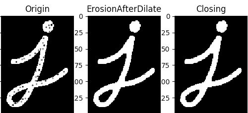
4 闭运算
顾名思义,开运算与闭运算是相反的语法糖——先膨胀再侵蚀,其作用也可以想象到了,可以填充上物体内部的杂点。
1 | def testClose(): |
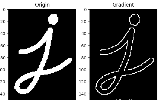
5.形态梯度
出现梯度变化的地方前景色保留,其它的去掉,用于检测边缘
1 | def testGradient(): |
6.tophat
顶帽 = 原图 - 开运算
开运算的效果是去除图像外的噪点,因此原图 - 开运算就得到了去掉的噪点。
通过API — morphologyEx(img, MORPH_TOPHAT, kernel)
1 | import cv2 |

7. blackhat
黑帽 = 原图 - 闭运算
闭运算可以将图形内部的噪声点去掉,那么原图 - 闭运算的结果就是图形内部的噪声点。
通过API — morphologyEx(img, MORPH_BLACKHAT, kernel)
1 | import cv2 |
8. 自定义内核
四、图像处理
图像金字塔
图像阈值操作
五、仿射变换
旋转(线性)
平移(向量加)
缩放(线性变换)
getAffineTransform
1 | warp_mat = getAffineTransform( srcTri, dstTri ); |
rotation
1 | rot_mat = getRotationMatrix2D( center, angle, scale ); |
轮廓
rectangle & boundingRect
然后利用cv2.rectangle(img, (x,y), (x+w,y+h), (0,255,0), 2)画出矩行
1 | 参数解释 |
1 | # 用绿色(0, 255, 0)来画出最小的矩形框架 |
七、Video api
1 | # 1、表示打开笔记本的内置摄像头, |
八、应用
Sobel导数
如何计算梯度,以及如何使用梯度来检测边缘。
Laplace算子
边缘检测算法。
Canny边缘检测
这儿是一个更高级的边缘检测算法。
霍夫线变换
霍夫变换来检测直线。
霍夫圆变换
霍夫变换来检测圆。
Remapping重映射
两副图像之间建立坐标位置的映射。
九、CV Face
CascadeClassifier
1 | haarcascade_eye.xml |
1、人脸检测
cv.CascadeClassifier
1 | # 人脸检测haarcascade_frontalface_default |
Dlib
人脸提取+关键点检测
CNN人脸检测模型名称: mmod_human_face_detector.dat.bz2
68维人脸检测模型名称: shape_predictor_68_face_landmarks.dat.bz2
5维人脸检测模型名称 shape_predictor_5_face_landmarks.dat.bz2
1 | detector = dlib.cnn_face_detection_model_v1(face_detector_model_path) # dlib.cnn_face_detection_model_v1 |
PyTorch Doc Detail
APIs
[TOC]
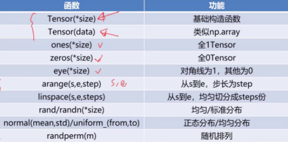
Tensor
pytorch
1 | #1 list->tensor |
libtorch(c++)
1 | //1 数组 -> Tensor |
张量操作
pytorch
1 | # index + slice |
libtorch(c++)
1 | // index |
3、 提取指定元素形成新的张量(关键字index:就代表是提取出来相应的元素组成新的张量)
1 | std::cout<<b.index_select(0,torch::tensor({0, 3, 3})).sizes();//选择第0维的0,3,3组成新张量[3,3,28,28] |
张量基本运算
3.1 pytorch
① 按元素的加减乘除正常使用±*/的运算符即可
② 矩阵乘法:例如xx^T
1 | x = torch.rand((3,4)) |
3.2 torchlib
① 按元素的加减乘除正常使用±*/的运算符即可
② 矩阵乘法:例如xx^T
1 | auto x = torch::rand({3,4}); |
Init Weight
1 | torch.nn.init.xavier_uniform_(conv.weight) |
API-tensor
torch — PyTorch 2.0 documentation
torch.reshape()
torch.reshape用来改变tensor的shape。
torch.reshape(tensor,shape)
tensor.squeeze()
维度压缩
如果 input 的形状为 (A×1×B×C×1×D),那么返回的tensor的形状则为 (A×B×C×D)
1 | x = torch.zeros(2, 1, 2, 1, 2) |
tensor.unsqueenze()
1 | x = torch.tensor([1, 2, 3, 4]) |
torch.gather函数
(todo)
图解PyTorch中的 []https://zhuanlan.zhihu.com/p/352877584
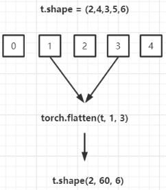
torch.flatten()
扁平化
torch.flatten(t, start_dim=0, end_dim=-1) 的实现原理如下。假设类型为 torch.tensor 的张量 t 的形状如下所示:(2,4,3,5,6),则 torch.flatten(t, 1, 3).shape 的结果为 (2, 60, 6)。将索引为 start_dim 和 end_dim 之间(包括该位置)的数量相乘【1,2,3维度的数据扁平化处理合成一个维度】,其余位置不变。因为默认 start_dim=0,end_dim=-1,所以 torch.flatten(t) 返回只有一维的数据。
mean()
求均值
var()
求方差
item()
.item()用于在只包含一个元素的tensor中提取值,注意是只包含一个元素,否则的话使用.tolist()
tolist()
tensor转换为Python List
permute
作用类似tf的transpose()
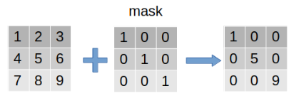
mask
pytorch提供mask机制用来提取数据中“感兴趣”的部分。过程如下:左边的矩阵是原数据,中间的mask是遮罩矩阵,标记为1的表明对这个位置的数据“感兴趣”-保留,反之舍弃。整个过程可以视作是在原数据上盖了一层mask,只有感兴趣的部分(值为1)显露出来,而其他部分则背遮住。
torch.masked_fill(input, mask, value)
参数:
- input:输入的原数据
- mask:遮罩矩阵
- value:被“遮住的”部分填充的数据,可以取0、1等值,数据类型不限,int、float均可
返回值:一个和input相同size的masked-tensor
使用:
- output = torch.masked_fill(input, mask, value)
- output = input.masked_fill(mask, value)
torch.masked_select(input, mask, out)
参数:
- input:输入的原数据
- mask:遮罩矩阵
- out:输出的结果,和原tensor不共用内存,一般在左侧接收,而不在形参中赋值
返回值:一维tensor,数据为“选中”的数据
使用:
- torch.masked_select(input, mask, out)
- output = input.masked_select(mask)
1 | selected_ele = torch.masked_select(input=imgs, mask=mask) # true表示selected,false则未选中,所以这里没有取反 |
torch.masked_scatter(input, mask, source)
说明:将从input中mask得到的数据赋值到source-tensor中
参数:
- input:输入的原数据
- mask:遮罩矩阵
- source:遮罩矩阵的”样子“(全零还是全一或是其他),true表示遮住了
返回值:一个和source相同size的masked-tensor
使用:
- output = torch.masked_scatter(input, mask, source)
- output = input.masked_scatter(mask, source)
API-Model
train(mode=True)
将module设置为 training mode。
仅仅当模型中有Dropout和BatchNorm是才会有影响。
eval()
将模型设置成evaluation模式
仅仅当模型中有Dropout和BatchNorm是才会有影响。
训练
BN使用注意事项
model.eval()之后,pytorch会管理BN的参数,所以不需要TF那般麻烦;
$$
Y = (X - running_mean) / sqrt(running_var + eps) * gamma + beta
$$
其中gamma、beta为可学习参数(在pytorch中分别改叫weight和bias),训练时通过反向传播更新;而running_mean、running_var则是在前向时先由X计算出mean和var,再由mean和var以动量momentum来更新running_mean和running_var。
所以在训练阶段,running_mean和running_var在每次前向时更新一次;
在测试阶段,则通过net.eval()固定该BN层的running_mean和running_var,此时这两个值即为训练阶段最后一次前向时确定的值,并在整个测试阶段保持不变。
torchrun
torchrun (Elastic Launch) — PyTorch 2.3 documentation
关于集群分布式torchrun命令踩坑记录(自用)-CSDN博客
Model Save & Load
save model
1 | torch.save({ |
save state_dict()
1 | torch.save(learner_model.get_model(position).state_dict(), model_weights_dir) |
Saving & Loading Model
Save:
1 | torch.save(model.state_dict(), PATH) |
Load:
1 | model = TheModelClass(*args, **kwargs) |
Save/Load Entire Model
Save:
1 | torch.save(model, PATH) |
Load:
1 | # Model class must be defined somewhere |
Export/Load Model in TorchScript Format
Export:
1 | model_scripted = torch.jit.script(model) # Export to TorchScript |
Load:
1 | model = torch.jit.load('model_scripted.pt') |
Saving & Loading a General Checkpoint for Inference and/or Resuming Training
Save:
1 | torch.save({ |
Load:
1 | model = TheModelClass(*args, **kwargs) |
Saving Multiple Models in One File
Save:
1 | torch.save({ |
Load:
1 | modelA = TheModelAClass(*args, **kwargs) |
Warmstarting Model Using Parameters from a Different Model
Saving & Loading Model Across Devices
Save:
1 | torch.save(modelA.state_dict(), PATH) |
Load:
1 | modelB = TheModelBClass(*args, **kwargs) |
Save on GPU, Load on CPU
Save:
1 | torch.save(model.state_dict(), PATH) |
Load:
1 | device = torch.device('cpu') |
Save on GPU, Load on GPU
Save:
1 | torch.save(model.state_dict(), PATH) |
Load:
1 | device = torch.device("cuda") |
Save on CPU, Load on GPU
Save:
1 | torch.save(model.state_dict(), PATH) |
Load:
1 | device = torch.device("cuda") |
Saving torch.nn.DataParallel Models
Save:
1 | torch.save(model.module.state_dict(), PATH) |
Load:
1 | # Load to whatever device you want |
模型参数(打印print)
1 | import torch |
此我们可以使用clone()方法来创建它们的副本。具体来说,我们可以使用clone()方法来创建一个张量的深拷贝,然后使用detach()方法来将其从计算图中分离,从而得到一个不会影响原始张量的新张量。
1 | # 打印模型的所有参数名和参数值,并取出参数值 |
tools_pandas APIs
[TOC]
数据初始化
1、readcsv
1 | df = pd.read_csv('file_path') |
2、
1 | df = pd.DataFrame(columns=['index', 'v2']) |
3、pd 和np转换
首先导入numpy模块、pandas模块、创建一个DataFrame类型数据df
1 | import numpy as np |
| 语法 | 操作 | 返回结果 |
|---|---|---|
df.head(n) |
查看 DataFrame 对象的前n行 | DataFrame |
df.tail(n) |
查看 DataFrame 对象的最后n行 | DataFrame |
df.sample(n) |
查看 n 个样本,随机 | DataFrame |
读取列
以下两种方法都可以代表一列:
1 | df['name'] # 会返回本列的 Series |
注意,当列名为一个合法的 python 变量时可以直接作为属性去使用。
读取部分行列
有时我们需要按条件选择部分列、部分行,一般常用的有:
| 操作 | 语法 | 返回结果 |
|---|---|---|
| 选择列 | df[col] |
Series |
| 按索引选择行 | df.loc[label] |
Series |
| 按数字索引选择行 | df.iloc[loc] |
Series |
| 使用切片选择行 | df[5:10] |
DataFrame |
| 用表达式筛选行 | df[bool_vec] |
DataFrame |
以上操作称为 Fancy Indexing(花式索引),它来自 Numpy,是指传递一个索引序列,然后一次性得到多个索引元素。Fancy Indexing 和 slicing 不同,它通常将元素拷贝到新的数据对象中。索引中可以有切片 slice,或者省略 ellipsis、新轴 newaxis、布尔数组或者整数数组索引等,可以看做是一个多维切片。
接下来我们将重点介绍一下这些查询的方法。
数据遍历
1. 使用 .iterrows()
iterrows() 方法返回 DataFrame 的索引标签和相应的行数据。这是一个迭代器,它会产生 (index, Series) 对,其中索引是行索引(如果有),Series 是该行的数据。
1 | import pandas as pd |
2. 使用 .itertuples()
itertuples() 方法返回一个迭代器,用于迭代 DataFrame 行作为命名元组。这种方式比使用 iterrows() 更快一些,因为不需要创建 Series 对象。
1 | # 遍历每一行 |
3. 使用 .apply()
apply() 方法可以应用于整个 DataFrame 或者沿着一个轴应用到每一列或每一行上。这里我们使用 axis=1 来对每一行应用函数。
1 | def process_row(row): |
4. 使用 .loc 或 .iloc
如果你想要更灵活地访问特定行或列的数据,可以使用 .loc 或 .iloc 方法。
1 | # 使用 .loc 按照标签索引访问 |
切片 [行/列]
我们可以像列表那样利用切片功能选择部分行的数据,但是不支持索引一条:
1 | df[:2] # 前两行数据 |
也可以选择列:
1 | df['name'] # 只要一列,Series |
按标签 .loc(行)
df.loc() 的格式为 df.loc[<索引表达式>, <列表达式>],表达式支持以下形式:
单个标签:
1 | # 代表索引,如果是字符需要加引号 |
单个列表标签:
1 | name, value, socre, grade |
1 | df.loc[[0,5,10]] # 指定索引 0,5,10 的行 |
带标签的切片,包括起始和停止start:stop, 可以其中只有一个,返回包括它们的数据:
1 | df.loc[0:5] # 索引切片, 代表0-5行,包括5 |
关于 loc 的更详细介绍可访问:loc 查询数据行和列。
进行切片操作,索引必须经过排序,意味着索引单调递增或者单调递减,以下代码中其中一个为 True,否则会引发 KeyError 错误。
1 | # 索引单调性 |
通过上边的规则可以先对索引排序再执行词义上的查询,如:
1 | # 姓名开头从 Ad 到 Bo 的 |
列筛选,必须有行元素:
1 | dft.loc[:, ['Q1', 'Q2']] # 所有行,Q1 和 Q2两列 |
按位置 .iloc
df.iloc 与 df.loc 相似,但只能用自然索引(行和列的 0 - n 索引),不能用标签。
1 | df.iloc[:3] |
如果想筛选多个不连续的行列数据(使用 np.r_),可以使用以下方法:
1 | # 筛选索引0-4&10&5-29每两行取一个&70-74 |
关于 iloc 的更详细介绍可访问:iloc 数字索引位置选择。
取具体值 .at
类似于 loc, 但仅取一个具体的值,结构为 at[<索引>,<列名>]:
1 | # 注:索引是字符需要加引号 |
同样 iat 和 iloc 一样,仅支持数字索引:
1 | df.iat[4, 2] # 65 |
.get 可以做类似字典的操作,如果无值给返回默认值(例中是0):
1 | df.get('name', 0) # 是 name 列 |
表达式筛选
[] 切片里可以使用表达式进行筛选:
1 | df[df['Q1'] == 8] # Q1 等于8 |
df.loc 里的索引部分可以使用表达式进行数据筛选。
1 | df.loc[df['Q1'] == 8] # 等于8 |
逻辑判断和函数:
1 | df.eq() # 等于相等 == |
其他函数:
1 | # isin |
函数筛选
函数生成具体的标签值或者同长度对应布尔索引,作用于筛选:
1 | df[lambda df: df['Q1'] == 8] # Q1为8的 |
函数不仅能应用在行位上,也能应用在列位上。
str查询
模糊查询
1 | data[data.列名.str.contains()] |
df内置方法
where 和 mask
1 | s.where(s > 90) # 不符合条件的为 NaN |
mask 和 where 还可以通过数据筛选返回布尔序列:
1 | # 返回布尔序列,符合条件的行为 True |
query
1 | df.query('Q1 > Q2 > 90') # 直接写类型 sql where 语句 |
filter
使用 filter 可以对行名和列名进行筛选。
1 | df.filter(items=['Q1', 'Q2']) # 选择两列 |
关于 filter 的详细介绍,可以查阅:Pandas filter 筛选标签。
索引选择器 pd.IndexSlice
pd.IndexSlice 的使用方法类似于df.loc[] 切片中的方法,常用在多层索引中,以及需要指定应用范围(subset 参数)的函数中,特别是在链式方法中。
1 | df.loc[pd.IndexSlice[:, ['Q1', 'Q2']]] |
复杂的选择:
1 | # 创建复杂条件选择器 |
按数据类型
可以只选择或者排除指定类型数据:
1 | df.select_dtypes(include=['float64']) # 选择 float64 型数据 |
any 和 all
any 方法如果至少有一个值为 True 是便为 True,all 需要所有值为 True 才为 True。它们可以传入 axis 为 1,会按行检测。
1 | # Q1 Q2 成绩全为 80 分的 |
理解筛选原理
df[<表达式>] 里边的表达式如果单独拿出来,可以看到:
1 | df.Q1.gt(90) |
会有一个由真假值组成的数据,筛选后的结果就是为 True 的内容。
mean() / median() / unique() / value_count()
mean()
median()
unique()
value_count()
map & apply
1 | # Series数据修改,返回当前列的series |
案例实操
获取指定值的索引
有时候我们需要知道指定值所在的位置,即一个值在表中的索引,可以使用以一下方法:
1 | # 指定值的的索引对 |
修改某行某列的值
1 | import pandas as pd |
相关内容
2020_PLAN
[TOC]
2020年专业精进
线性代数
麻省理工公开课:线性代数 http://open.163.com/newview/movie/courseintro?newurl=M6V0BQC4M
矩阵的秩–挺适合预习线性代数的https://zhuanlan.zhihu.com/p/108093909
图形学变换
会议:
[CVPR 2019 论文大盘点—人体姿态篇](https://bbs.cvmart.net/topics/531/CVPR 2019 Human Pose))
AI基础知识
专业书籍
- 《图形学基础》
AI 集成项目学习
- CenterNet
- InsightFace
- 梳理基础知识点
- SMPL*
- 关于 骨骼动画之理解蒙皮算法https://blog.csdn.net/smsmn/article/details/53870334
tools_np Doc
[TOC]
np初始化
np.arange()
np.random
1 | # random.randn(x1, x2, x3, ...) |
np.meshgrid()
生成网格点坐标矩阵
np.eye()
函数的原型:numpy.eye(N,M=None,k=0,dtype=<class ‘float’>,order=’C)
返回的是一个二维2的数组(N,M),对角线的地方为1,其余的地方为0.
参数介绍:
(1)N:int型,表示的是输出的行数
(2)M:int型,可选项,输出的列数,如果没有就默认为N
(3)k:int型,可选项,对角线的下标,默认为0表示的是主对角线,负数表示的是低对角,正数表示的是高对角。
(4)dtype:数据的类型,可选项,返回的数据的数据类型
(5)order:{‘C’,‘F’},可选项,也就是输出的数组的形式是按照C语言的行优先’C’,还是按照Fortran形式的列优先‘F’存储在内存中
案例:(普通的用法)
1 | import numpy as np |
1 | [[1. 0. 0.] |
高级用法:
1 | import numpy as np |
np.identity()
这个函数和之前的区别在于,这个只能创建方阵,也就是N=M
函数的原型:np.identity(n,dtype=None)
参数:n,int型表示的是输出的矩阵的行数和列数都是n
dtype:表示的是输出的类型,默认是float
返回的是nxn的主对角线为1,其余地方为0的数组
1 | import numpy as np |
np.ravel()
np.expand_dims()
1 | import numpy as np |
方式2
1 | import numpy as np |
np.sequeeze()
1 | import numpy as np |
另一种方式
1 | import numpy as np |
np.flatten()
两者的功能是一致的,将多维数组降为一维,但是两者的区别是返回拷贝还是返回视图
np.flatten()返回一份拷贝,对拷贝所做修改不会影响原始矩阵,
np.ravel()返回的是视图,修改时会影响原始矩阵
1 | import numpy as np |
1 | b: [1 2 3 4] |
allclose
1 | numpy.allclose(a, b, rtol=1e-05, atol=1e-08, equal_nan=False)[source] |
eg: 判断两个数据的误差小于2:
1 | np.allclose(a, b, atol=2) |
这两个数据,可以是相同维度的,例如
1 | a = [149.820974 188.13338026 145.44900513] |
diag
np.argmax()
1 | import numpy as np |
https://wenku.baidu.com/view/1d3dbe48ac1ffc4ffe4733687e21af45b307fe78.html
https://blog.csdn.net/weixin_38145317/article/details/79650188
np.where()
np.where(condition, x, y)
满足条件(condition),输出x,不满足输出y。
如果是一维数组,相当于[xv if c else yv for (c,xv,yv) in zip(condition,x,y)]
1 | >>> aa = np.arange(10) |
np.where(condition)
只有条件 (condition),没有x和y,则输出满足条件 (即非0) 元素的坐标 (等价于numpy.nonzero)。这里的坐标以tuple的形式给出,通常原数组有多少维,输出的tuple中就包含几个数组,分别对应符合条件元素的各维坐标。
1 | a = np.array([2,4,6,8,10]) |
1 | bid_history = [0, 1, 2, 0, 2] |
np.repeat
1 | a = np.zeros(54, dtype=np.int8) |
Slice
:: (逆向序列)
1 | a = np.arange(10) |
1 | [0 1 2 3 4 5 6 7 8 9] |
statck相关
stack() Join a sequence of arrays along a new axis.
vstack() Stack along first axis. == np.concatenate(tup, axis=0)
hstack() Stack along second axis. (column wise). == np.concatenate(tup, axis=1)
dstack() Stack arrays in sequence depth wise (along third dimension).==np.concatenate(tup, axis=2)
concatenate() Join a sequence of arrays along an existing axis.
np.stack()
np.hstack()
np.vstack()
np.dstack()
np.concatenate()
np.split()
np.hsplit
np.vsplit
np.dsplit
1 | split : 1D; indices_or_sections ``[2, 3]`` would, for ``axis=0``, result in |
1 | import numpy as np |
Out:
1 | (4, 3) |
np矩阵运算:
mean 均值
var 方差
item
dot
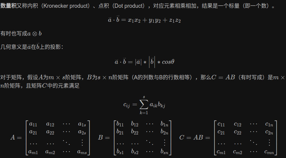
数量积又称内积(Kronecker product)、点积(Dot product),对应元素相乘相加,结果是一个标量(即一个数)。
cross
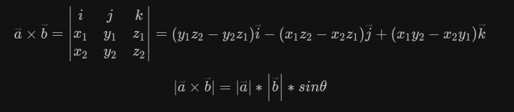
向量积又称外积、叉积(Cross product)
multiply或*
普通乘积:对应元素相乘,结果还是向量。
np.linalg
np.linalg.norm 求范数
序列化NP
bcolz
1 | Write: |
https://vimsky.com/zh-tw/examples/detail/python-method-bcolz.carray.html
pickle
path相关
glob模块是最简单的模块之一,内容非常少。用它可以查找符合特定规则的文件路径名。跟使用windows下的文件搜索差不多。查找文件只用到三个匹配符:””, “?”, “[]”。””匹配0个或多个字符;”?”匹配单个字符;”[]”匹配指定范围内的字符,如:[0-9]匹配数字。
1 | import glob |
Point Set Matching/Registration Benchmark
[Point Set Matching/Registration Benchmark](http://gwang-cv.github.io/2019/05/01/Point Set Matching-Registration Benchmark/)
A list of point set matching/registration resources collected by Gang Wang. If you find that important resources are not included, please feel free to contact me.
Point Set Matching/Registration Material
POINT SET MATCHING/REGISTRATION METHODS [WIKI]
Point Matching/Registration Methods
- [MCT] A mathematical analysis of the motion coherence theory, IJCV’1989 [pdf]
- [ICP: point-to-point] Method for Registration of 3-D Shapes, Robotics-DL tentative’1992 [pdf] [code][code] [code] [material] [tutorial]
- [ICP: point-to-plane] Object modeling by registration of multiple range images, IVC’1992 [pdf]
- [ICP] Iterative point matching for registration of free-form curves and surfaces, IJCV’1994 [pdf]
- [RPM/Softassign] New algorithms for 2d and 3d point matching: pose estimation and correspondence, PR’1998 [pdf] [code]
- [MultiviewReg] Multiview registration for large data sets, 3DDIM’1999 [pdf]
- [SC] Shape matching and object recognition using shape contexts, TPAMI’2002 [pdf][wiki] [project] [code]
- [EM-ICP] Multi-scale EM-ICP: A Fast and Robust Approach for Surface Registration, ECCV’2002 [pdf] [code]
- [LM-ICP] Robust registration of 2D and 3D point sets, IVC’2003 [pdf] [code]
- [TPS-RPM] A new point matching algorithm for non-rigid registration, CVIU’2003 [pdf] [project] [code]
- [Survey] Image registration methods: a survey, IVC’2003 [pdf]
- [KCReg] A correlation-based approach to robust point set registration, ECCV’2004 [pdf] [code]
- [3DSC] Recognizing objects in range data using regional point descriptors, ECCV’2004 [pdf] [code_pcl]
- [RGR] Robust Global Registration, ESGP’2005 [pdf]
- [RPM-LNS] Robust point matching for nonrigid shapes by preserving local neighborhood structures, TPAMI’2006 [pdf] [code]
- [IT-FFD] Shape registration in implicit spaces using information theory and free form deformations, TPAMI’2006 [pdf]
- [Rigid] Rigid Body Registration, 2007 [ch02]
- [CDC] Simultaneous covariance driven correspondence (cdc) and transformation estimation in the expectation maximization framework, CVPR’2007 [pdf] [project]
- [Nonrigid-ICP] Optimal step nonrigid icp algorithms for surface registration, CVPR’2007 [pdf] [code] [code]
- [GNA] Global non-rigid alignment of 3D scans, TOG’2007 [pdf]
- [PF] Particle filtering for registration of 2D and 3D point sets with stochastic dynamics, CVPR’2008 [pdf]
- [JS] Simultaneous nonrigid registration of multiple point sets and atlas construction, TPAMI’2008 [pdf]
- [4PCS] 4-points congruent sets for robust pairwise surface registration, TOG’2008 [pdf] [project]
- [GICP] Generalized ICP, RSS’2009 [pdf] [code]
- [MP] 2D-3D registration of deformable shapes with manifold projection, ICIP’2009 [pdf]
- [SMM] The mixtures of Student’s t-distributions as a robust framework for rigid registration, IVC’2009 [pdf]
- [Algebraic-PSR] An Algebraic Approach to Affine Registration of Point Sets, ICCV’2009 [pdf]
- [SM] Subspace matching: Unique solution to point matching with geometric constraints, ICCV’2009 [pdf]
- [FPFH] Fast Point Feature Histograms (FPFH) for 3D Registration, ICRA’2009 [pdf] [code]
- [GO] Global optimization for alignment of generalized shapes, CVPR’2009 [pdf]
- [ISO] Isometric registration of ambiguous and partial data, CVPR’2009 [pdf]
- [GF] A new method for the registration of three-dimensional point-sets: The Gaussian fields framework, IVC’2010 [pdf]
- [RotInv] Rotation invariant non-rigid shape matching in cluttered scenes, ECCV’2010 [pdf] [code]
- [CDFHC] Group-wise point-set registration using a novel cdf-based havrda-charvát divergence, IJCV’2010 [pdf] [code]
- [QPCCP] A quadratic programming based cluster correspondence projection algorithm for fast point matching, CVIU’2010 [pdf] [code]
- [CPD] Point set registration: Coherent point drift, NIPS’2007 [pdf] TPAMI’2010 [pdf] [code]
- [PFSD] Point set registration via particle filtering and stochastic dynamics, TPAMI’2010 [pdf]
- [ECMPR] Rigid and articulated point registration with expectation conditional maximization, TPAMI’2011 [pdf] [project] [code]
- [GMMReg/TPS-L2] Robust point set registration using gaussian mixture models, NIPS’2005 TPAMI’2011 [pdf] [code]
- [TPRL] Topology preserving relaxation labeling for nonrigid point matching, TPAMI’2011 [pdf]
- [OOH] Robust point set registration using EM-ICP with information-theoretically optimal outlier handling, CVPR’2011 [pdf]
- [SGO] Stochastic global optimization for robust point set registration, CVIU’2011
- [survey] 3D Shape Registration, 3DIAA’2012
- [Multiview LM-ICP] Accurate and automatic alignment of range surfaces, 3DIMPVT’2012 [pdf] [code]
- [ISC] Intrinsic shape context descriptors for deformable shapes, CVPR’2012 [pdf]
- [RPM-Concave] Robust point matching revisited: A concave optimization approach, ECCV’2012 [pdf] [code]
- [RINPSM] Rotation Invariant Nonrigid Point Set Matching in Cluttered Scenes, TIP’2012 [pdf] [code]
- [RPM-L2E] Robust estimation of nonrigid transformation for point set registration, CVPR’2013 [pdf] [code]
- [GO-ICP] Go-ICP: Solving 3D Registration Efficiently and Globally Optimally, ICCV’2013 [pdf] TPAMI’2016 [pdf] [code]
- [Survey] Registration of 3D point clouds and meshes: a survey from rigid to nonrigid, TVCG’2013 [[pdf]](https://orca.cf.ac.uk/47333/1/ROSIN registration of 3d point clouds and meshes.pdf)
- [NMM] Diffeomorphic Point Set Registration Using Non-Stationary Mixture Models, ISBI’2013 [pdf]
- [Sparse-ICP] Sparse Iterative Closest Point, ESGP’2013 [pdf] [project] [code]
- [JRMPC] A Generative Model for the Joint Registration of Multiple Point Sets, ECCV’2014 [pdf] [project] [code&data]
- [RPM-VFC] Robust Point Matching via Vector Field Consensus, TIP’2014 [pdf] [code]
- [GLTP] Non-rigid Point Set Registration with Global-Local Topology Preservation, CVPRW’2014 [pdf]
- [color-GICP] Color supported generalized-ICP, VISAPP’2014 [pdf]
- [RPM-Concave] Point Matching in the Presence of Outliers in Both Point Sets: A Concave Optimization Approach, CVPR’2014 [pdf] [code]
- [super4PCS] Super 4pcs fast global pointcloud registration via smart indexing, CGF’2014 [pdf] [code] [OpenGR]
- [SDTM] A Riemannian framework for matching point clouds represented by the Schrodinger distance transform, CVPR’2014 [pdf]
- [GLMD-TPS] A robust global and local mixture distance based non-rigid point set registration, PR’2015 [pdf] [code]
- [CSM] Non-rigid point set registration via coherent spatial mapping, SP’2015 [pdf]
- [ADR] An Adaptive Data Representation for Robust Point-Set Registration and Merging, ICCV’2015 [pdf]
- [MLMD] MLMD: Maximum likelihood mixture decoupling for fast and accurate point cloud registration, 3DV’2015 [pdf] [project]
- [APSR] Non-rigid Articulated Point Set Registration for Human Pose Estimation, WACV’2015 [pdf]
- [RegGF] Non-rigid visible and infrared face registration via regularized Gaussian fields criterion, PR’2015 [pdf] [code]
- [LLT] Robust feature matching for remote sensing image registration via locally linear transforming, TGRS’2015 [pdf] [code]
- [RPM-L2E] Robust L2E estimation of transformation for non-rigid registration, TSP’2015 [pdf] [code]
- [GLR] Robust Nonrigid Point Set Registration Using Graph-Laplacian Regularization, WACV’2015 [pdf]
- [FPPSR] Aligning the dissimilar: A probabilistic method for feature-based point set registration, ICPR’2016 [pdf]
- [IPDA] Point Clouds Registration with Probabilistic Data Association, IROS’2016 [pdf] [code]
- [CPPSR] A probabilistic framework for color-based point set registration, CVPR’2016 [pdf] [project]
- [GOGMA] GOGMA: Globally-optimal gaussian mixture alignment, CVPR’2016 [pdf]
- [GO-APM] An Efficient Globally Optimal Algorithm for Asymmetric Point Matching, TPAMI’2016 [pdf] [project] [code]
- [PR-GLS] Non-Rigid Point Set Registration by Preserving Global and Local Structures, TIP’2016 [pdf] [code]
- [conreg] Non-iterative rigid 2D/3D point-set registration using semidefinite programming, TIP’2016 [pdf]
- [PM] Probabilistic Model for Robust Affine and Non-rigid Point Set Matching, TPAMI’2016 [pdf]
- [SPSR] A Stochastic Approach to Diffeomorphic Point Set Registration With Landmark Constraints, TPAMI’2016 [pdf]
- [FRSSP] Fast Rotation Search with Stereographic Projections for 3D Registration, TPAMI’2016 [pdf]
- [VBPSM] Probabilistic Model for Robust Affine and Non-rigid Point Set Matching, TPAMI’2016 [pdf] [code]
- [MFF] Image Correspondences Matching Using Multiple Features Fusion, ECCV’2016 [pdf] [code]
- [FGR] Fast Global Registration, ECCV’2016 [pdf] [code]
- [HMRF ICP] Hidden Markov Random Field Iterative Closest Point, arxiv’2017 [pdf] [code]
- [SSFR] Global Registration of 3D LiDAR Point Clouds Basedon Scene Features: Application toStructured Environments, RS’2017 [pdf]
- [color-PCR] Colored point cloud registration revisited, ICCV’2017 [pdf]
- [dpOptTrans] Efficient Globally Optimal Point Cloud Alignment using Bayesian
Nonparametric Mixtures, CVPR’2017 [pdf] [code] - [GORE] Guaranteed Outlier Removal for Point Cloud Registration with Correspondences, TPAMI’2017 [pdf]
- [CSGM] A systematic approach for cross-source point cloud registration by preserving macro and micro structures, TIP’2017 [pdf]
- [FDCP] Fast descriptors and correspondence propagation for robust global point cloud registration, TIP’2017 [pdf]
- [RSWD] Multiscale Nonrigid Point Cloud Registration Using Rotation-Invariant Sliced-Wasserstein Distance via Laplace-Beltrami Eigenmap, SIAM JIS’2017 [pdf]
- [MR] Non-Rigid Point Set Registration with Robust Transformation Estimation under Manifold Regularization, AAAI’2017 [pdf] [code]
- [LPM] Locality Preserving Matching, IJCAI’2017 [pdf] IJCV’2019 [pdf] [code]
- [DARE] Density adaptive point set registration, CVPR’2018 [pdf] [code]
- [GC-RANSAC] Graph-Cut RANSAC, CVPR’2018 [pdf] [code]
- [3D-CODED] 3D-CODED: 3D correspondences by deep deformation, ECCV’2018 [pdf] [project] [code]
- [3DFeat-NET] 3dfeat-net: Weakly supervised local 3d features for point cloud registration, ECCV’2018 [pdf] [code]
- [MVDesc-RMBP] Learning and Matching Multi-View Descriptors for Registration of Point Clouds, ECCV’2018 [pdf]
- [SWS] Nonrigid Points Alignment with Soft-weighted Selection, IJCAI’2018 [pdf]
- [DLD] Dependent landmark drift: robust point set registration with aGaussian mixture model and a statistical shape model, arxiv’2018 [pdf] [code]
- [DeepMapping] DeepMapping: Unsupervised Map Estimation From Multiple Point Clouds, arxiv’2018 [pdf] [project]
- [APSR] Adversarial point set registration, arxiv’2018 [pdf]
- [3DIV] Fast and Globally Optimal Rigid Registration of 3D Point Sets by Transformation Decomposition, arxiv’2018 [pdf]
- [Analysis] Analysis of Robust Functions for Registration Algorithms, arxiv’2018 [pdf]
- [MVCNN] Learning Local Shape Descriptors from Part Correspondences with Multiview Convolutional Networks, TOG’2018 [pdf] [project]
- [CSCIF] Cubature Split Covariance Intersection Filter-Based Point Set Registration, TIP’2018 [pdf]
- [FPR] Efficient Registration of High-Resolution Feature Enhanced Point Clouds, TPAMI’2018 [pdf]
- [DFMM-GLSP] Non-rigid point set registration using dual-feature finite mixture model and global-local structural preservation, PR’2018 [pdf]
- [PR-Net] Non-Rigid Point Set Registration Networks, arxiv’2019 [pdf] [code]
- [SDRSAC] SDRSAC: Semidefinite-Based Randomized Approach for Robust Point Cloud Registration without Correspondences, arxiv’2019 [pdf] [code]
- [3DRegNet] 3DRegNet: A Deep Neural Network for 3D Point Registration, arxiv’2019 [pdf]
- [PointNetLK] PointNetLK: Robust & Efficient Point Cloud Registration using PointNet, arxiv’2019 [pdf] [code]
- [RPM-MR] Nonrigid Point Set Registration with Robust Transformation Learning under Manifold Regularization, TNNLS’2019 [pdf] [code]
- [FGMM] Feature-guided Gaussian mixture model for image matching, PR’2019 [pdf]
- [LSR-CFP] Least-squares registration of point sets over SE (d) using closed-form projections, CVIU’2019 [pdf]
- [FilterReg] FilterReg: Robust and Efficient Probabilistic Point-Set Registration using Gaussian Filter and Twist Parameterization, CVPR’2019 [pdf] [project] [code]
- [TEASER] A Polynomial-time Solution for Robust Registration with Extreme Outlier Rates, arxiv’2019 [pdf]
Mismatch Removal Methods
- [RANSAC] Random sample consensus: a paradigm for model fitting with applications to image analysis and automated cartography, 1981 [pdf] [wiki]
- [MLESAC] MLESAC: A new robust estimator with application to estimating image geometry, CVIU’2000 [pdf] [code_pcl]
- [PROSAC] Matching with PROSAC-progressive sample consensus, CVPR’2005 [pdf] [code_pcl]
- [ICF/SVR] Rejecting mismatches by correspondence function, IJCV’2010 [pdf]
- [GS] Common visual pattern discovery via spatially coherent correspondences, CVPR’2010 [[pdf]](http://www.jdl.ac.cn/project/faceId/paperreading/Paper/Common Visual Pattern Discovery via Spatially Coherent Correspondences.pdf) [code]
- [VFC] A robust method for vector field learning with application to mismatch removing, CVPR’2011 [pdf] [code]
- [DefRANSAC] In defence of RANSAC for outlier rejection in deformable registration, ECCV’2012 [[pdf]](https://media.adelaide.edu.au/acvt/Publications/2012/2012-In Defence of RANSAC for Outlier Rejection in Deformable Registration.pdf) [code]
- [CM] Robust Non-parametric Data Fitting for Correspondence Modeling, ICCV’2013 [pdf] [code]
- [AGMM] Asymmetrical Gauss Mixture Models for Point Sets Matching, CVPR’2014 [pdf]
- [TC] Epipolar geometry estimation for wide baseline stereo by Clustering Pairing Consensus, PRL’2014 [pdf]
- [BF] Bilateral Functions for Global Motion Modeling, ECCV’2014 [pdf] [project] [code]
- [WxBS] WxBS: Wide Baseline Stereo Generalizations, BMVC’2015 [pdf] [project]
- [RepMatch] RepMatch: Robust Feature Matching and Posefor Reconstructing Modern Cities, ECCV’2016 [pdf] [project] [code]
- [SIM] The shape interaction matrix-based affine invariant mismatch removal for partial-duplicate image search, TIP’2017 [pdf] [code]
- [DSAC] DSAC: differentiable RANSAC for camera localization, CVPR’2017 [pdf] [code]
- [GMS] GMS: Grid-based Motion Statistics for Fast, Ultra-robust Feature Correspondence, CVPR’2017 [pdf] [code]
- [LMI] Consensus Maximization with Linear Matrix Inequality Constraints, CVPR’2017 [pdf] [project] [code]
- [LFGC] Learning to Find Good Correspondences, CVPR’2018 [pdf] [code]
- [GC-RANSAC] Graph-Cut RANSAC, CVPR’2018 [pdf] [code]
- [SRC] Consensus Maximization for Semantic Region Correspondences, CVPR’2018 [pdf] [code]
- [CODE] Code: Coherence based decision boundaries for feature correspondence, TPAMI’2018 [pdf] [project]
- [LPM] Locality preserving matching, IJCV’2019 [pdf] [code]
- [LMR] LMR: Learning A Two-class Classifier for Mismatch Removal, TIP’2019 [pdf] [code]
- [PFFM] Progressive Filtering for Feature Matching, ICASSP’2019 [pdf]
- [NM-Net] NM-Net: Mining Reliable Neighbors for Robust Feature Correspondences, arXiv’2019 [pdf]
Graph Matching Methods
- [SM] A spectral technique for correspondence problems using pairwise constraints, ICCV’2005 [pdf] [code]
- [SM-MAP] Efficient MAP approximation for dense energy functions, ICML’2006 [pdf] [code]
- [SMAC] Balanced Graph Matching, NIPS’2006 [pdf] [code]
- [FCGM] Feature correspondence via graph matching: Models and global optimization, ECCV’2008 [pdf]
- [PM] Probabilistic Graph and Hypergraph Matching, CVPR’2008 [pdf]
- [IPFP] An Integer Projected Fixed Point Method for Graph Matching and MAP Inference, NIPS’2009 [pdf] [code]
- [RRWM] Reweighted Random Walks for Graph Matching, ECCV’2010 [pdf]
- [FGM] Factorized graph matching, CVPR’2012 [pdf] [code]
- [DGM] Deformable Graph Matching, CVPR’2013 [pdf] [code]
- [MS] Progressive mode-seeking on graphs for sparse feature matching, ECCV’2014 [pdf] [code]
Misc
- [RootSIFT] Three things everyone should know to improve object retrieval, CVPR’2012 [pdf] [related code]
- [DM-CNN] Descriptor Matching with Convolutional Neural Networks: a Comparison to SIFT, arXiv’2014 [pdf]
- [DASC] DASC: Robust Dense Descriptor for Multi-modal and Multi-spectral Correspondence Estimation, TPAMI’2017 [pdf] [project]
- [MODS] MODS: Fast and Robust Method for Two-View Matching, CVIU’2015 [pdf] [project] [code]
- [Elastic2D3D] Efficient Globally Optimal 2D-to-3D Deformable Shape Matching, CVPR’2016 [pdf] [project]
- [TCDCN] Facial Landmark Detection by Deep Multi-task Learning, ECCV’2014 [pdf] [project]
- [LAI] Object matching using a locally affine invariant and linear programming techniques, TPAMI’2013 [pdf]
- [GeoDesc] GeoDesc: Learning Local Descriptors by Integrating Geometry Constraints, ECCV’2018 [pdf] [code]
Deep Features
- [TFeat] Learning local feature descriptors with triplets and shallow convolutional neural networks, BMVC’2016 [pdf] [code]
- [L2-Net] L2-Net: Deep Learning of Discriminative Patch Descriptor in Euclidean Space, CVPR’2017 [pdf] [code]
- [HardNet] Working hard to know your neighbor’s margins: Local descriptor learning loss, CVPR’2018 [pdf] [code]
- [AffNet] Repeatability Is Not Enough: Learning Discriminative Affine Regions via Discriminability, ECCV’2018 [pdf] [code]
APPLICATIONS
Remote Sensing Image Registration
- [GLPM] Guided Locality Preserving Feature Matching for Remote Sensing Image Registration, TGRS’2018 [pdf]
Retinal Image Registration
- [DB-ICP] The dual-bootstrap iterative closest point algorithm with application to retinal image registration, TMI’2003 [pdf]
- [GDB-ICP] Registration of Challenging Image Pairs: Initialization, Estimation, and Decision, TPAMI’2007 [pdf] [project]
- [ED-DB-ICP] The edge-driven dual-bootstrap iterative closest point algorithm for registration of multimodal fluorescein angiogram sequence, TMI’2010 [pdf]
Palmprint Image Registration
- Robust and efficient ridge-based palmprint matching, TPAMI’2012 [pdf]
- Palmprint image registration using convolutional neural networks and Hough transform, arxiv’2019 [pdf]
Visual Homing Navigation
- Visual Homing via Guided Locality Preserving Matching, ICRA’2018 [pdf]
HDR Imaging
- Locally non-rigid registration for mobile HDR photography, CVPRW’2015 [pdf]
Misc
- Hand Motion from 3D Point Trajectories and a Smooth Surface Model, ECCV’2004 [pdf] [project]
- A robust hybrid method for nonrigid image registration, PR’2011 [pdf]
- Aligning Images in the Wild, CVPR’2012 [pdf] [code]
- Robust feature set matching for partial face recognition, CVPR’2013 [pdf]
- Multi-modal and Multi-spectral Registrationfor Natural Images, ECCV’2014 [pdf] [project]
- Articulated and Generalized Gaussian KernelCorrelation for Human Pose Estimation, TIP’2016 [pdf]
- Infrared and visible image fusion via gradient transfer and total variation minimization, Information Fusion’2016 [pdf] [code]
DATABASES
General databases
- 2D Synthesized Chui-Rangarajan Dataset (deformation, noise, and outliers)
- TOSCA
- Multi-View Stereo Dataset
- Multi-View Stereo for Community Photo Collections
- Multi-View Stereo
- VGG Affine Datasets
- Multi-view VGG’s Dataset
- Oxford Building Reconstruction
- IMM Datasets
- MPEG7 CE Shape-1 Part B
- [Leaf Shapes Database](http://www.imageprocessingplace.com/downloads_V3/root_downloads/image_databases/leaf shape database/leaf_shapes_downloads.htm)
- CMU House/Hotel Sequence Images
- Generated Matching Dataset
- Image Sequences
- Mythological creatures 2D
- Tools 2D
- Human face
- Cars & Motorbikes
- DIML Multimodal Benchmark
- Street View Dataset [github] [data]
- EVD: Extreme View Dataset [EVD_tentatives] [EZD]
- WxBS: Wide Baseline Dataset [W1BS]
- Stanford 3D Scanning
- MPI FAUST Dataset
- Mikolajczyk Database
- Panoramic Image Database
- PS-Dataset (A Large Dataset for improving Patch Matching, PhotoSynth Dataset for improving local patch Descriptors)
- Two-view Geometry
- Point clouds data sets for 3D registration
- IMW CVPR 2019: Challenge
- Robotic 3D Scan Repository
- Database for 3D surface registration
Other databases
- FIRE: Fundus Image Registration Dataset
- DRIVE (Retinal Images)
- DRIONS-DB (Retinal Images)
- STARE (Retinal Images)
- Plant Images
- MR Prostate Images
- CV Images
- ETHZ Datasets
- CVPapers
- YACVID
- Intelligent remote sensing data analyis
TOOLS
- VLFeat
- PCL: Point Cloud Library
- Pointmatcher: a modular library implementing the ICP algorithm for aligning point clouds
- Open3D: A Modern Library for 3D Data Processing
- 3D keypoints (MeshDOG) and local descriptors (MeshHOG)
- COLMAP
- OpenMVG: open Multiple View Geometry
- VisualSFM : A Visual Structure from Motion System
- Medical Image Registration Toolbox
- Graph Matching Toolbox in MATLAB
- FAIR: Flexible Algorithms for Image Registration [pdf]
- Range Image Registration Toolbox